How to use Score-P suite to profile the code.
- Author
- N. Ohana
- Date
- 06/2017
Prepare the code
Load Score-P module
The module Score-P has to be loaded.
On Piz Daint, it is named Score-P/3.0-Cray[XXX]-2016.11, where [XXX] stands for Intel, CCE, PGI or GNU.
On Marconi, it is included in the module scalasca/2.3.1.
- Note
- With Intel, there is a 'bug' during the linking stage so you need to enter the following command:
export LD_LIBRARY_PATH=$LD_LIBRARY_PATH:/opt/cray/pe/papi/5.5.0.1/lib either in the terminal or add it to your .bashrc file.
Compile the code for profiling
Using the generic makefile, change the value of PROFILE from FALSE to TRUE and compile the code using the standard make command. This will produce a binary named orb5bin_PROFILE that can be launched using the same command as the usual binary.
User-defined regions
If you want to instrument a specific part of the code, you should use the profiler module. Simply add profiler_begin_region(name) and profiler_end_region(name) where name is a generic name around the code of interest.
- Attention
- Calls to
profiler_begin_region(name) and profiler_end_region(name) must be correctly nested, otherwise the execution will fail.
- Warning
- The total number of regions is currently limited to 128.
- Note
- For performance purpose, the less visited regions the better. Thus one should avoid placing regions inside loops, around is preferable.
Run the code
You can edit your job script to specify what kind of measurement you are interested in. Insert the following lines before the srun command:
export SCOREP_EXPERIMENT_DIRECTORY=[name]
sets the location of the profiler output,
export SCOREP_ENABLE_PROFILING=[true/false]
tells whether you want to profile the code execution (i.e. accumulate the information over region calls),
export SCOREP_ENABLE_TRACING=[true/false]
tells whether you want to trace the code execution (i.e. record the full timeline of each region entered and exited),
- Note
- Tracing experiments produce much larger output files, and they increase with the number of timesteps of the simulation. You should deactivate it if you don't need it.
export SCOREP_METRIC_PAPI=[comma-separated list]
sets the list of device-specific counters you want to track. For instance, PAPI_LD_INS is the number of load instructions, PAPI_SR_INS is the number of store instructions, PAPI_L2_TCM is the cache miss of level 2, ... You can run the command papi_avail to see the list of available counters on your hardware and their description.
The srun command does not need to be modified, except that it should call the right executable (orb5bin_PROFILE).
Report analysis
Once you have run the code, it is recommended to run some post-processing analysis, which derives additional metrics from the recorded ones such as splitting computation/communication/idle time. For this, load Scalasca module (Scalasca/2.3.1-Cray[XXX]-2016.11 on Piz Daint and scalasca/2.3.1 on Marconi) and use the command:
> square -s $SCOREP_EXPERIMENT_DIRECTORY
(You may want to add it in your job script.)
- Note
- If you are using Cray programming environment on Piz Daint, you have to load Scalasca module for PGI or Intel (it is currently not available for CCE) and this will swap your programming environment. It is not a problem since you don't need to recompile anything.
You are now ready to analyze the profiling and/or tracing reports.
Profiling report
Cube GUI
In order to visualize the report, use the command:
> cube $SCOREP_EXPERIMENT_DIRECTORY/summary.cubex
(or profile.cubex if you have not run the post-processing analysis, but less information will be available.)
The interface looks like:
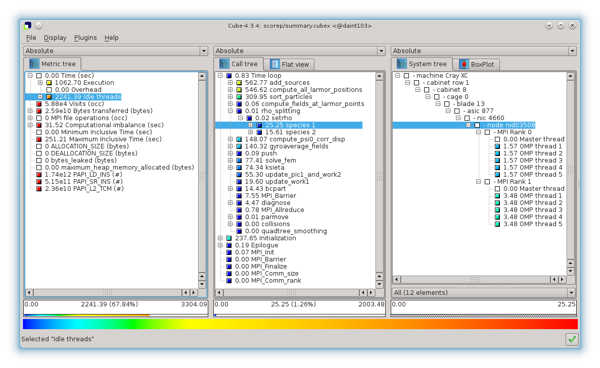
Cube interface
Three trees are displayed:
- the metric tree, in which you can select a quantity of interest,
- the region tree, in which you can select an instrumented region,
- the system tree, in which you can select a particular computing element.
Values are aggregated from rightmost to leftmost panel, with presentation in center and right panes based on selections from the left. Metric values in the left panel are aggregates of every selected region in the central panel from every process or thread selected in the right panel.
Each tree node name is preceded by its inclusive value if it is collapsed, or exclusive value if it is expanded.
Many hiding and sorting options are offered by right-clicking on any panel. For instance, one can detect the slowest regions by selecting Execution time on the metric panel, and Right click → Sort tree items... → Sort by inclusive value (descending) on the region panel.
A useful tool is the BoxPlot tab of the right panel, which provides statistics over all processes and threads.
Command-line
If you want to display basic information in a terminal (for instance at the end of your job script), you can use:
> cube_stat $SCOREP_EXPERIMENT_DIRECTORY/summary.cubex -
p -% -r
"Time loop"MetricRoutine Count Sum Mean Variance Minimum Quartile 25 Median Quartile 75 Maximum
time INCL(Time loop) 12 3014.543567 251.211964 0.000000 251.211881 251.211899 251.211948 251.211979 251.212155
time EXCL(Time loop) 12 0.993102 0.082759 0.006553 0.005252 0.030050 0.113682 0.155988 0.160265
time MPI_Barrier 12 9.055266 0.754606 0.620504 0.000420 0.028353 0.507575 1.323278 1.508791
time sort_particles 12 371.943708 30.995309 0.028106 30.834799 30.940379 31.102672 31.155819 31.155819
time
update_work1 12 23.522664 1.960222 0.000426 1.940460 1.953459 1.973441 1.979984 1.979984
time compute_fields_at_larmor_points 12 332.679388 27.723282 0.043375 27.523808 27.531257 27.657992 27.873576 27.922725
time gyroaverage_fields 12 168.381618 14.031802 0.000037 14.025957 14.029801 14.035711 14.037646 14.037646
time
compute_psi0_corr_disp 12 177.682008 14.806834 0.002933 14.754986 14.789090 14.841515 14.858682 14.858682
time
push 12 134.806962 11.233913 0.001675 11.194733 11.220954 11.259403 11.272136 11.273094
time
ksieta 12 89.211096 7.434258 0.009604 7.340432 7.343907 7.403526 7.505005 7.528084
time
parmove 12 0.011796 0.000983 0.000000 0.000962 0.000976 0.000997 0.001004 0.001004
time rho_splitting 12 192.123043 16.010254 0.994941 15.055225 15.090595 15.697420 16.730340 16.965384
time
solve_fem 12 92.894190 7.741182 4.459814 5.719262 7.049236 9.093623 9.763103 9.763103
time
bcpart 12 17.311638 1.442636 0.260569 0.953909 0.972010 1.282556 1.811148 1.931364
time
add_sources 12 675.318972 56.276581 0.000000 56.276202 56.276216 56.276457 56.276867 56.276960
time
collisions 12 0.002922 0.000244 0.000000 0.000239 0.000242 0.000247 0.000248 0.000248
time
quadtree_smoothing 12 0.000360 0.000030 0.000000 0.000027 0.000029 0.000032 0.000033 0.000033
time MPI_Allreduce 12 0.936390 0.078032 0.006617 0.000151 0.003035 0.052523 0.136757 0.155914
time
diagnose 12 5.363082 0.446924 0.071883 0.190227 0.359076 0.618625 0.703620 0.703620
subroutine, public diagnose(step, step_tot, time)
Definition: diagnostics.F90:97
subroutine update_work1(iter, work1)
Definition: efluid.F90:372
subroutine push(zdt)
Definition: examples.F90:923
subroutine, public solve_fem(time)
Solve potential equations and compute field vector.
Definition: fields.F90:4178
type(collisions_variables) collisions
Definition: globals.F90:346
subroutine ksieta(iact)
Store particle's position in or .
Definition: onestep.F90:307
subroutine update_pic1_and_work2(iter)
Definition: onestep.F90:441
subroutine, public compute_psi0_corr_disp(run_on_device)
Definition: part.F90:7224
subroutine compute_all_larmor_positions(isp, pic1_loc, pic2_loc, npart_loc)
Definition: part.F90:2492
subroutine bcpart(pic1_loc, npart_loc, isp, run_on_device)
Boundary Conditions at s=sfmax (and s=sfmin if needed) and periodicity at phi=2pi.
Definition: part.F90:1734
subroutine, public parmove(iter, run_on_device, work1flag, work2flag, work3flag, work5flag, work6flag, work7flag, work8flag, work9flag)
Definition: part.F90:2241
integer, save p
Spline order.
Definition: pdespline.F90:30
subroutine, public quadtree_smoothing(part, npart, pos1min, pos1max, pos2min, pos2max, sigma, maxppc, do_2w, diagnose, diagnose_array)
Definition: quadtree.F90:322
subroutine, public add_sources(step)
Add various source terms to the RHS of Vlasov/Boltzmann equation.
Definition: sources.F90:89
Multiple files comparison
Unfortunately, it is hard to get a visual comparison of different simulations with Score-P tools. This problem can be overcame with the Matlab script matlab/performance_analysis/hist_timings.m in the git repository.
This script plots an histogram all subtimings of any instrumented region for different simulations. One can thus vary one parameter (e.g. number of OpenMP threads) for different configurations (e.g. with/without sorting).
Here is an example of such scan:
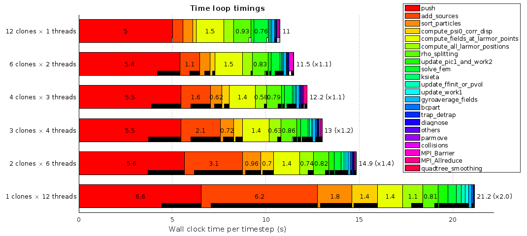
Matlab figure for multiple files comparison
The white bars indicate the time spent in MPI routines (not visible here because it is a single node case), while the black ones indicate the OpenMP threads idle time.
Tracing report
not written yet
Vampir GUI
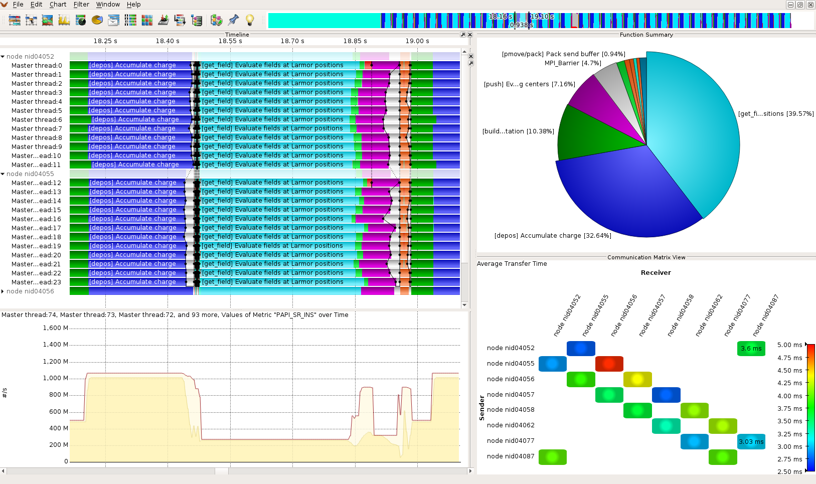
Vampir interface
References
Score-P Documentation
Scalasca User Guide
CUBE Display Quick Reference
 1.9.4 on Wed May 7 2025